Tutorial | Network Analysis with R - Manipulating Network Data
[Tutorial Network-Analysis R Visualization Author: Jinhang Jiang
Student Researcher at University of Kansas, Business Analytics
Introduction
Network analysis is a technique that uses graph theory to study complex real-world problems,
such as computational biology, engineering, finance, marketing, neuroscience, political science, and public health (Kolaczyk et al., 2014).
In my previous works, I have done quite a lot of network analysis in the python environment with NetworkX and node2vec.
However, recently I came across the book - “Statistical Analysis of Network Data with R”
(this is the 1st version, and the 2nd version was published in 2020)-
written by Eric D. Kolaczyk and Gábor Csárdi, which showed me many cool packages (e.g., igraph) in R
which provides high-quality network analysis in terms of manipulating graphs, descriptive analysis, mathematical modeling, statistical modeling, etc.
The book came with a list of code demos, which can be found here: https://github.com/kolaczyk/sand.
This blog is built upon Chapter 2 of the book: Manipulating Network Data, assuming that you already understood the basic concepts of network analysis,
such as nodes, edges, etc. However, if you need a comprehensive explanation, I encourage you to read the book.
What you need:
RStudio (or similar IDEs) and “igraph” (an R package, available in CRAN)
In case you do not have “igraph” installed:
  ## Download and install the package
install.packages("igraph")

## Load package
library(igraph)
Code
Create Undirected and Directed Graphs
To manually create a graph, the function “graph.formula” can be used.
To make it more understandable for creating directed graphs, I proposed an airport network consisting of three airports:
JFK (New York City airport), PEK (Beijing airport), and CDG (Paris airport).
Thus, the directed graph that I created can be read: we only have one-way flights from JFK to PEK and CDG (assume some travel restrictions applied);
PEK and CDG are mutually connected, and you can fly both ways.
Get Basic Info of the Graphs
To make the blog concise, the rest of the demo will only focus on undirected graphs. For more reference, please visit the book’s GitHub repository.
A graph, represented by G = (V, E), is a mathematical structure consisting of a set V of vertices and a set E of edges.
The number of vertices and the number of edges in the graph are sometimes called the order and size of graph G (Kolaczyk et al., 2014).
You may use V(graph) and E(graph) to check the vertices and edges; use vcount(graph) and ecount(graph) to check the order and size of the graph; use print_all(graph) to show the summary of the graph.
Visualize the graph
You may use the command of plot(graph) to visualize the graph:
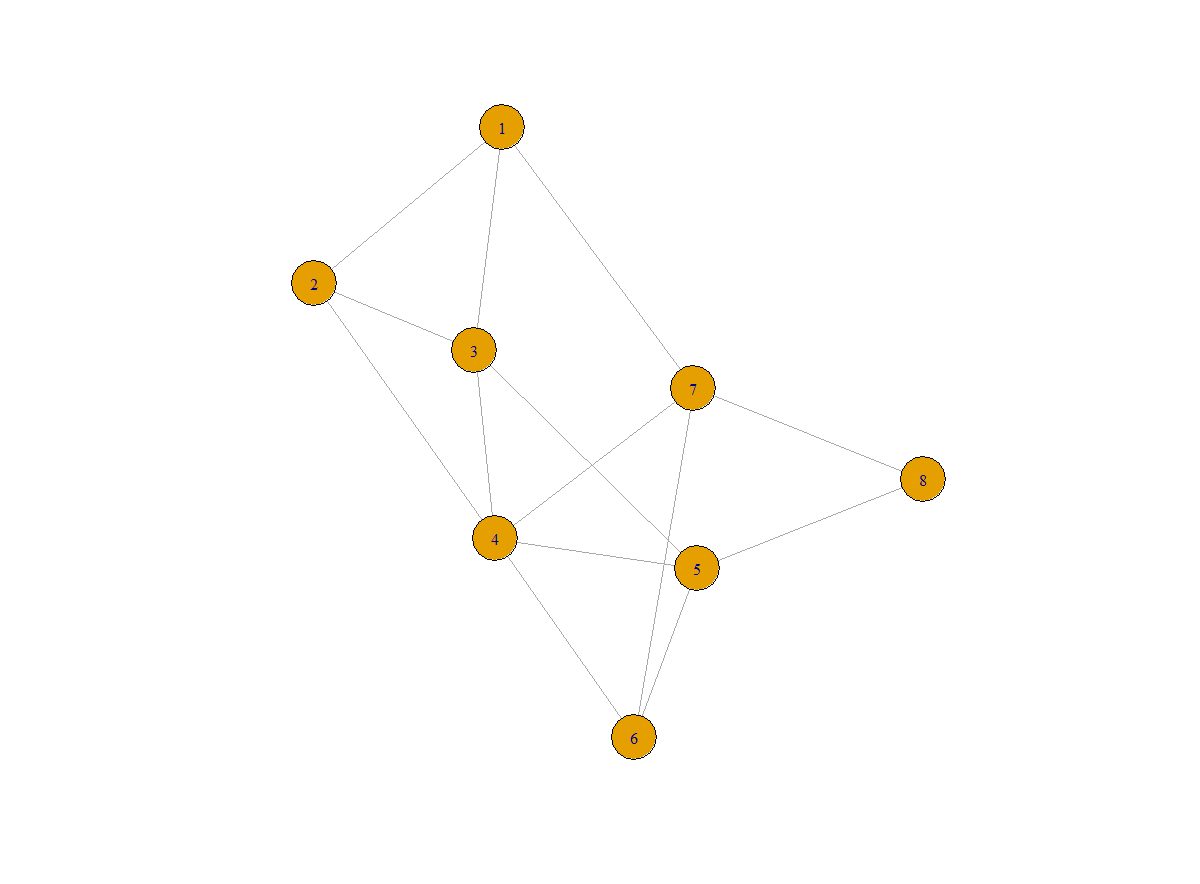
Figure 1. plot(g)
Label the vertices
I made the graph whose vertices were labeled with numbers 1 through N. In practice, you might already have natural labels, such as names. So here is how you could label your vertices and how it would look like:
V(g)$name <- c("Adam","Judy","Bobby","Sam","Frank","Jay","Tom","Jerry")
plot(g)
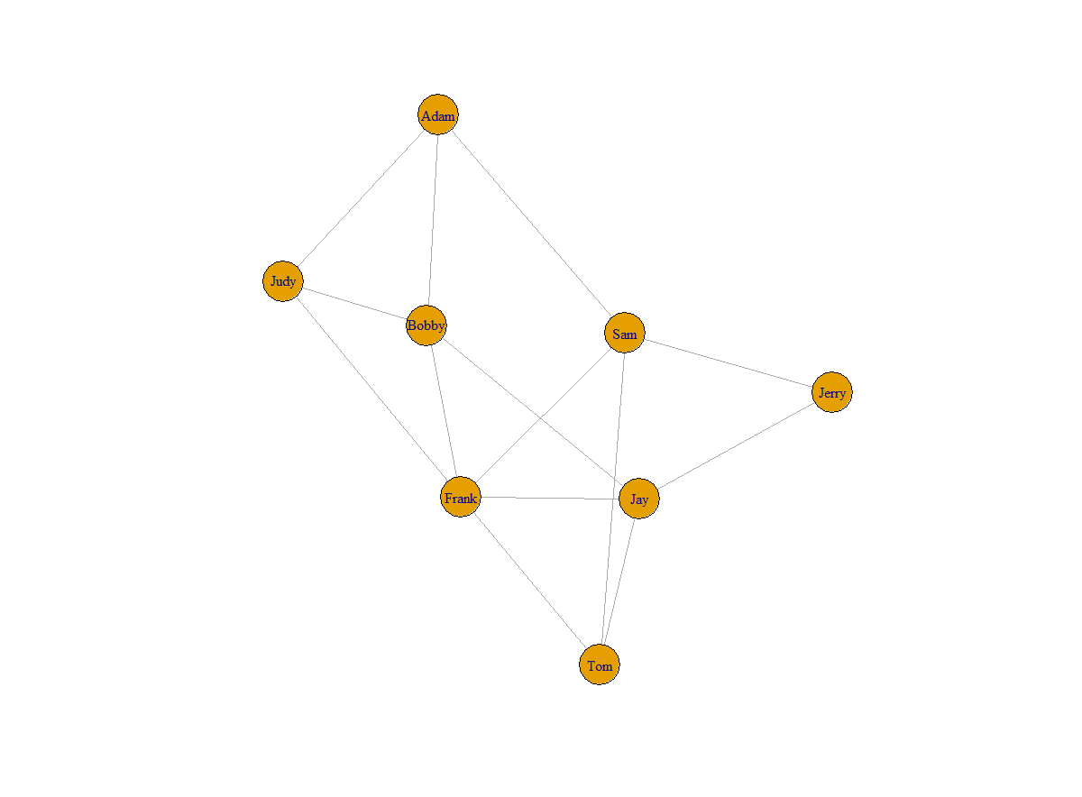
Figure 2: Labeled graph
Representations for Graphs
Normally, the graph will be stored in three basic formats: adjacency lists, edge lists, and adjacency matrix (Kolaczyk et al., 2014).
An adjacency list is a collection of unordered lists. Each unordered list describes the set of neighbors of a specific vertex in the graph within an adjacency list.
This format is what igraph uses in the graph summary function.
An edge list is a two-column table to list all the node pairs in the graph. This format is preferred by NetworkX (in python).
The adjacency matrix’s entries show whether two vertices in the graph are connected or not. If there is a link between two nodes, “i and j,” the row-column indices (i, j) will be marked as 1, otherwise 0. Therefore, the adjacency matrix will be symmetric for undirected graphs.
Statistical models normally prefer to encode graphs with this format, such as node2vec which requires the adjacency matrix as inputs.
You can use the functions of get.adjlist(graph), get.edgelist(graph), and get.adjacency(graph) to get the three different formats, respectively.
Operations on Graphs
In practice, we might want to remove certain edges or join graphs to get subgraphs. In this case, the math operators can help you achieve the goal.
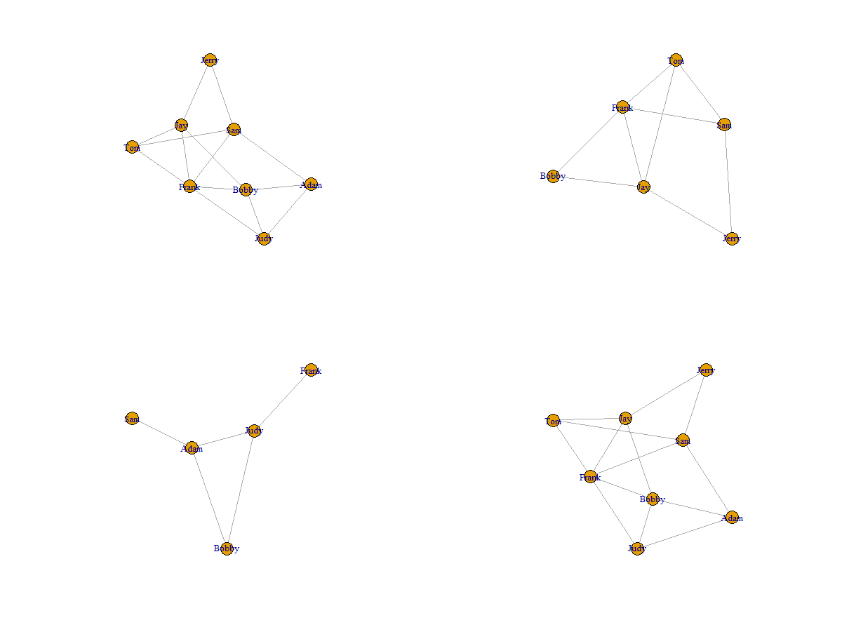
Figure 3. Operations on graphs
The graph in (1, 1) is the original graph. The graph in (1, 1) removed two vertices from the original graph.
The graph in (2, 1) is made of certain edges (the edges were removed from the original graph due to the removal of vertices).
The graph in (2, 2) is the joined graph of (1, 1) and (2, 1), and it has the same structure as (1, 1).
Using Data Frames
In real-world problems, we rarely make graphs manually. Instead, we have to import data.
For the best practice to manipulate graphs, we normally need to prepare two data files/data frames.
One of the files needs to contain all the attributes for each vertex in the graph.
The other file needs to contain the edges in the network (typically an edge list).
In the book, the author gave an example of a lawyer dataset of Lazega. The information is stored in two different files: elist.lazega and v.attr.lazega.
The original data is available in the sand (Statistical Analysis of Network Data) library. Therefore, here is how you would read your own data:
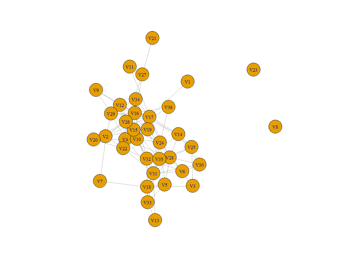
Figure 4. Read your own data
Conclusion
In this blog, I covered the code for creating directed and undirected graphs, visualizing graphs, getting statistics from graphs, labeling vertices, generating different formats of representations, subsetting and joining graphs, and reading your own network data with igraph.
Relevant Readings
NetworkX: Code Demo for Manipulating Subgraphs
Analyzing Disease Co-occurrence Using NetworkX, Gephi, and Node2Vec
Reference
Statistical Analysis of Network Data with R, by Eric D. Kolaczyk and Csárdi Gábor, Springer, 2014, pp. 13–28.
