Author: Jinhang Jiang, Maren Olson

Contributors: Andrew Aviles, Tzu Hsuan Chang

Master of Science in Business Analytics at Arizona State University, Class 2021

Project Summary

This project provided by Kaggle included a dataset of 79 explanatory variables describing aspects of residential homes in Ames, Iowa. You may find all the data sources and description of the project at here.

The goal of this competition was to predict the final sales price for each home listed. We did this problem because we were looking to apply our regression techniques as well as our stacking and exploratory data analysis skills. This problem set allowed us to use all of the above practices. Moreover, the datasets contain many missing values, which offered us the opportunity to gain experience in handling missing data.

We ran multiple regression techniques such as XGB regressor, SGD regressor, MLP regressor, Decision Tree regressor, Random Forest regressor, CatBoost regressor, Light GBM, and SVR. We stacked some together and experimented to see which ones ended up with the smallest Root-Mean-Squared-Error.

The prediction that we submitted was two columns (Figure 1.1). The first column was the ID of the house and the second column was our predicted sales price. The prediction is scored based on the Root-Mean-Squared-Error between the predicted value logarithm and the log of the observed sales price. The smallest RMSE was the best prediction. After running base models and the tuned models, we found that our tubed CatBoost regression model got us the lowest score of 0.12392 of RMSE, which was 863rd place (out of 4525) on the Leaderboard.

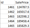
Figure1.1 - Sample of Submission

Data

- Overview

The competition offered us two datasets to work on. One of them is the training data with 1460 observations and 81 columns, which contains each house’s ID and the sale price. The other dataset is the holdout file, which includes 1459 observations.

We first looked into the types of features of the training dataset. Figure 2.1 shows that the whole dataset has 43 categorical features and 36 numeric variables, including “ID”.

Figure2.1 - The Numbers of Numeric & Categorical Features

Then, we took the efforts to detect if there were any missing values in the dataset. In the training dataset, 19 variables have missing values. The holdout dataset has 33 features with missing values. Some features have very high percentages of missing values. For example, the feature, PoolQC (Pool Quality), has as high as 99.5% missing values. Features like PoolQC, may hurt the accuracy of the prediction model and lead us to invalid conclusions. So, we removed the features with at least 80% of the values that are missing. The details are explained in the Data Processing section.

Before we started to process the data, we also studied the necessary statistical information of the 38 numeric features. In Figure 2.2, we found out that the ranges of some features, like the SalePrice, are relatively large. Many regression models we were going to use would need us to do some types of transformations of those features before processing.

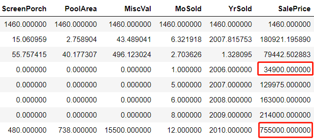
Figure2.2 - Statistical Info of All the Numeric Variables

- Data Processing

Missing values always hurt the accuracy of the prediction models. Before we did any transformations, we decided to check out for the columns with at least 80% of values missing first. According to Figure 2.3, there are four variables with a large number of missing values, and they were “Alley”, “PoolQC”, “Fence”, and “MiscFeature”.

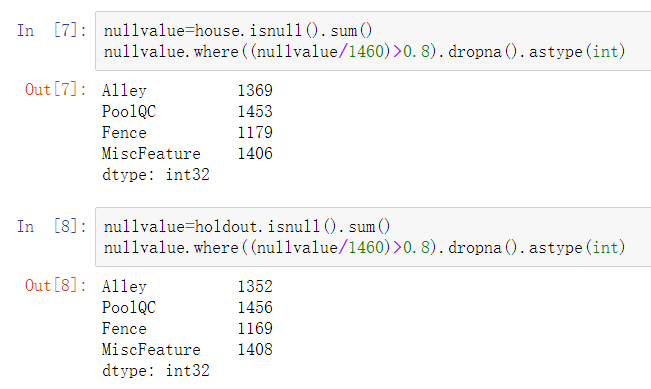
Figure2.3 - The Variables With At Least 80% Missing Values

Making sure we made the same changes to the training dataset and holdout dataset was essential in processing the data. The difference in the number of columns in each dataset, inconsistent data formats, and the unmatched number of values in the categorical variables would all possibly cause troubles to our models. Therefore, to better prepare the data and make sure any transformations will reflect on both the training dataset and holdout dataset, we used the code in Figure 2.4 to combine those two datasets together temporarily with labels 0 and 1, and the code for splitting the dataset back to the original dataset is also provided.

Figure2.4 - Code for Combine and Uncombine the Datasets

For all the categorical variables, we converted them to dummy variables to deal with the missing values. For all the missing values in the numeric variables, we filled them with the average of the current variable.

- Feature Engineering

We also created a few new variables based on the existing variables. For example, we used the data about when the house was renovated and when it was sold to generate a new variable called “AgeofHouse”, which helped us intuitively understand the relationship between the house prices and the quality of the house.

Figure2.5 - New Feature “AgeofHouse”

We wondered if we needed to do a log transformation for the “SalePrice” since it contains some relatively large values that would have a negative impact on the accuracy of the models. And the Residuals vs Fitted plots (Figure 2.6 and Figure 2.7) before and after the log transformation confirmed our assumption that the transformation made the model more linear.

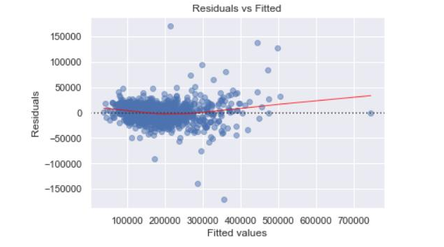
Figure2.6 - Residual vs Fitted Before Log Transformation

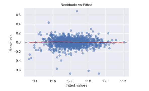
Figure2.7 - Residual vs Fitted After Log Transformation

- Plots for Correlation

We created some plots to study the data. We first looked at the correlation between the target variable and the rest of the variables. Figure 2.8 shows the top 30 features in terms of absolute correlation with SalePrice of the house. The dark color indicates the variable is negatively correlated with SalePrice.

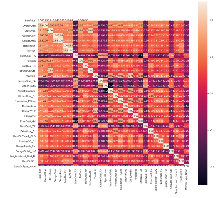
Figure2.8 - Top 30 “Most” Correlated Variables

We also took a look at the relationship between the “SalePrice” and the individual variables in detail. We selected several interesting charts to present in this report. For example, we made a scatter plot (Figure 2.9) regarding the “SalePrice” and “AgeofHouse”, the feature we created in the previous step. As we can see, the newer the house, the more likely for the house to be sold at a higher price. Thus, we are confident that the houses with prices over $500,000 were either built or renovated within the most recent 15 years.

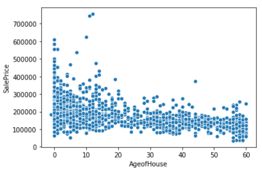
Figure2.9 - AgeofHouse vs. SalePrice

Another example is the plot for “OverallQual” and “SalePrice”. “OverallQual” is the variable that is most positively related to the “SalePrice”, and the plot (Figure 2.10) clearly shows that the higher ratings will lead to higher prices.

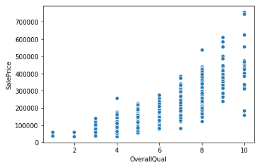
Figure2.10 - OverallQual vs. SalePrice

Our final training dataset has 1460 observations and 289 variables; and the holdout dataset has 1459 observations and 289 variables.

Modeling

- Individual Models Performance (base vs. tuned model)

Nine regression models were selected in this case:
OLS, XGBRegressor, SGDRegressor
DecisionTreeRegressor, RandomForestRegressor, SVR
CatBoostRegressor, LightGBM, MLPRegressor.

We used the OLS as our base model, and we generated the regression results of the model in the Figure 3.1：

Figure3.1 - OLS Regression Results

According to the OLS report, we learned that the R-squared is 0.943 which means 94.3% of “SalePrice” can be explained by the independent variables in the model. The kaggle score for this model is 0.15569.

In the following table (Figure 3.2), we list kaggle scores for all the models with both untuned and tuned parameters. CatBoostRegressor with tuned parameters had the best performance, 0.12392, among all the other models. This score put us at the number 863 out of 4525 teams (equivalently to the top 19%) by the time we wrote this report.

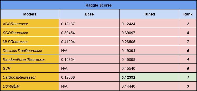
Figure3.2 - Table for Kaggle Scores

- Stacking Models and Average Ensembles

We also created several stacking models and average ensemble models. These types of models normally can help reduce the error by having multiple models work together. However, none of these models can outperform CatboostRegressor. The output is listed in the Figure 3.3:

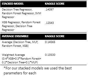
Figure3.3 - Kaggle Scores for Stacking and Average Ensemble Models

Conclusion

Overall, our main challenge with the “House Prices Advanced Regression Techniques” problem was that there was an ample amount of missing data. We tested the data with multiple solutions for missing value, but it was still hard to find a way to improve the accuracy of the models dramatically. Also, we believed that if we could have a bigger training dataset, it may also help improve the models.

After submitting various models, we noticed that our tuned CatBoost regression model was the best predictor of the house prices. We also ran four stacked and average ensemble models composed of three or more different tuned regression models, but none scored better than the CatBoost regressor.

We found this project interesting because we are using many different explanatory variables to predict a single price. This was also interesting because we can use the same methods on datasets from other cities or states to predict house pricing and compare the average prices of different locations. We could also use prediction models like this to help with future house market sales prices.

---

---